Introgression

Jerome Kelleher and Konrad Lohse

There has been great interest in understanding the contributions past populations have made to the genetic diversity of current populations via admixture. In particular, the availability of whole genome sequence data from archaic hominins (Green et al., 2010) has allowed geneticists to identify admixture tracks (Sankararaman, 2016). In the simplest case, admixture tracts can be defined heuristically as regions of the genome that show excessive similarity between a putative source and a recipient population (usually quantified relative to some non-admixed reference population, see Durand et al., 2011). Because recombination breaks down admixture tracts, their length distribution gives a clock for calibrating admixture and this information has been used to date the admixure contributions Neanderthals and other archaic hominins have made to non-African modern human populations (Sankararamanm 2016)

Crucially, the power to identify admixture depends on the relative time between the admixture event and the earlier divergence between source and recipient population: the shorter this interval, the harder it is to detect admixture. This is because samples from the source and recipient poulations are increasingly likely to share local ancestry regardless of recent admixture. In other words, it becomes increasingly difficult to distinguish admixture from incomplete lineage sorting (ILS).

In the following section we use msprime simulations to ask what fraction of admixture tracts are identifiable as such.

To illustrate this, we simulate genetic ancestry under a very simple toy history of divergence and admixture which is loosely motivated by the demographic history of modern humans and Neanderthals. As suggested in other tutorial material, we will first examine properties of the resulting tree sequence directly, rather than use it to simulate mutations. We assume a minimal sample of a single (haploid) genome from a modern human population in Africa and Eurasia as well as an ancient Neanderthal sample.

In the resulting tree sequence we want to distinguish three categories of segments: i) tracts actually involved in Neanderthal admixture, ii) the subset of those tracts in which the Eurasian and Neanderthal lineages we have sampled coalesce within the Neanderthal population and iii) segments at which the Eurasian and Neanderthal lineages are more closely related to each other than either are to the African lineage. The last category is interesting because it is the only one that can be unambiguously detected in data (via derived mutations that are shared by Neanderthals and Eurasians). However, while it must include all of ii), it also contains an additional set of short tracts that are due to ILS.

First we set up a highly simplified demographic history of human+Neanderthal demography and simulate a single chromosome of 20Mb in length:

import random
import collections

import matplotlib.pyplot as plt
import msprime
import numpy as np

def run_simulation(sequence_length, random_seed=None):
    time_units = 1000 / 25  # Conversion factor for kya to generations
    demography = msprime.Demography()
    # The same size for all populations; highly unrealistic!
    Ne = 10**4
    demography.add_population(name="Africa", initial_size=Ne)
    demography.add_population(name="Eurasia", initial_size=Ne)
    demography.add_population(name="Neanderthal", initial_size=Ne)

    # 2% introgression 50 kya
    demography.add_mass_migration(
        time=50 * time_units, source='Eurasia', dest='Neanderthal', proportion=0.02)
    # Eurasian 'merges' backwards in time into Africa population, 70 kya
    demography.add_mass_migration(
        time=70 * time_units, source='Eurasia', dest='Africa', proportion=1)
    # Neanderthal 'merges' backwards in time into African population, 300 kya
    demography.add_mass_migration(
        time=300 * time_units, source='Neanderthal', dest='Africa', proportion=1)

    ts = msprime.sim_ancestry(
        recombination_rate=1e-8,
        sequence_length=sequence_length,  
        samples=[
            msprime.SampleSet(1, ploidy=1, population='Africa'),
            msprime.SampleSet(1, ploidy=1, population='Eurasia'),
            # Neanderthal sample taken 30 kya
            msprime.SampleSet(1, ploidy=1, time=30 * time_units, population='Neanderthal'),
        ],
        demography = demography,
        record_migrations=True,  # Needed for tracking segments.
        random_seed=random_seed,
    )
    print(f"Simulation of {sequence_length/10**6}Mb run, using record_migrations=True")
    print(
        "NB: time diff from Neanderthal split to admixture event is",
        f"{300 * time_units - 50 * time_units:.0f} gens",
        f"({(300 * time_units - 50 * time_units) / 2 / Ne} coalescence units)"
    )
    return ts

ts = run_simulation(20 * 10**6, 1)

Simulation of 20.0Mb run, using record_migrations=True
NB: time diff from Neanderthal split to admixture event is 10000 gens (0.5 coalescence units)

The record_migrations option allows us to track segments of ancestral material that migrate from the Eurasian population into the Neanderthal population (backwards in time). We can then examine the length distributions of these segments and compare them with the length of the segments that also go on to coalesce within the Neanderthal population.

def get_migrating_tracts(ts):
    neanderthal_id = [p.id for p in ts.populations() if p.metadata['name']=='Neanderthal'][0]
    migrating_tracts = []
    # Get all tracts that migrated into the neanderthal population
    for migration in ts.migrations():
        if migration.dest == neanderthal_id:
            migrating_tracts.append((migration.left, migration.right))
    return np.array(migrating_tracts) 

def get_coalescing_tracts(ts):
    neanderthal_id = [p.id for p in ts.populations() if p.metadata['name']=='Neanderthal'][0]
    coalescing_tracts = []
    tract_left = None
    for tree in ts.trees():
        # 1 is the Eurasian sample and 2 is the Neanderthal
        mrca_pop = ts.node(tree.mrca(1, 2)).population
        left = tree.interval[0]
        if mrca_pop == neanderthal_id and tract_left is None:
            # Start a new tract
            tract_left = left      
        elif mrca_pop != neanderthal_id and tract_left is not None:
            # End the last tract
            coalescing_tracts.append((tract_left, left))
            tract_left = None
    if tract_left is not None:
        coalescing_tracts.append((tract_left, ts.sequence_length))
    return np.array(coalescing_tracts)

def get_eur_nea_tracts(ts):
    tracts = []
    tract_left = None
    for tree in ts.trees():
        # 1 is the Eurasian sample and 2 is the Neanderthal
        mrca = tree.mrca(1, 2)
        left = tree.interval[0]
        if mrca != tree.root and tract_left is None:
            # Start a new tract
            tract_left = left      
        elif mrca == tree.root and tract_left is not None:
            # End the last tract
            tracts.append((tract_left, left))
            tract_left = None
    if tract_left is not None:
        tracts.append((tract_left, ts.sequence_length))
    return np.array(tracts)

                                    
migrating = get_migrating_tracts(ts)
within_nea = get_coalescing_tracts(ts)
eur_nea = get_eur_nea_tracts(ts)

We build three different lists. The first is the set of tracts that exist in the Eurasian genome because they have come from Neanderthals via admixture at time \(T_{ad}\) (be careful here: in reverse time terminology, we denote the “source” population as Eurasian and the “destination” population as Neanderthals). This is done simply by finding all migration records in which the “destination” population name is Neanderthal. The second list (which must contain a subset of the segments in the first list) is the ancestral segments that went on to coalesce within the Neanderthal population. The third list contains all segments in which the Eurasian and Neanderthal sample coalesce before their ancestor coalesces with the African sample. The third list includes both Eurasian segments of Neanderthal origin and segments that did not migrate but coalesce further back in time than the Neanderthal-Human population split at \(T_{split}\).

migrating_l = migrating[:,1] - migrating[:,0]
print(f"There are {len(migrating_l)} migrating tracts of total length {np.sum(migrating_l)}")
migrating_total = np.sum(migrating_l)
within_nea_total = np.sum(within_nea[:,1] - within_nea[:,0])
nea_eur_closest = np.sum(eur_nea[:,1] - eur_nea[:,0])
totals = np.array([migrating_total, within_nea_total, nea_eur_closest])
print("Total lengths:", totals)
print("Proportions:", totals/ts.sequence_length)

There are 5 migrating tracts of total length 373730.0
Total lengths: [ 373730.  165617. 4475561.]
Proportions: [0.0186865  0.00828085 0.22377805]

The total length of admixed segments is about 1.9% of the chromosome, which accords with our migration fraction of \(f=0.02\) (although since this is only made up of 5 tracts, we might expect considerable random variation in this percentage). We expect a proportion \(1-e^{-(T_{split}-T_{ad})}\) of admixed lineages to coalesce, where \(T_{split}\) and \(T_{ad}\) are measured in coalescence units of \(2 N_e\) generations. We have assumed a split time of 300kya, an admixture time of 50kya and a generation time of 25 years. Given these time parameters and \(N_e =10000\), \(T_{split}-T_{ad} = 1/2\), so we expect \(1 -(e^{-1/2})=0.39\) of admixed sequence to coalesce in the Neanderthal population. The actual observed proportion is 165617/373730 = 0.44, which isn’t far off. However, the fraction of the genome which shows the Eurasian and the Neanderthal as each others closest relatives is much higher (over 20%): most of this must therefore be ILS.

How about the lengths of the tracts? We can plot these out in histogram form.

kb = 1 / 1000
plt.hist([
    migrating_l * kb,   
    (within_nea[:,1] - within_nea[:,0]) * kb,    
    (eur_nea[:,1] - eur_nea[:,0]) * kb,],
    label=["Migrating", "Within NEA", "EUR-NEA closest"]
)
plt.yscale('log')
plt.legend()
plt.xlabel("Tract length (KB)");

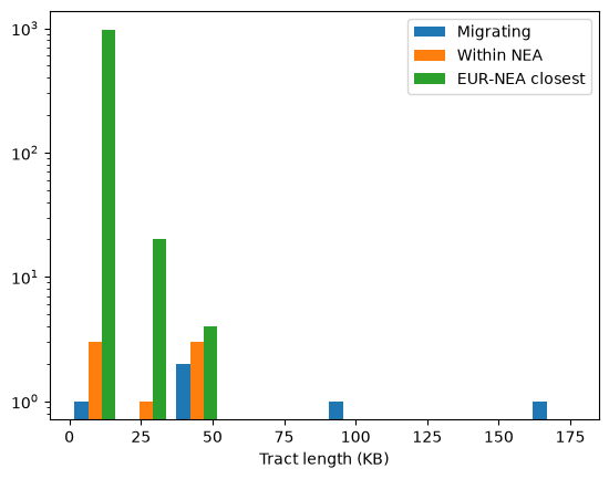
Note that this is just a single replicate: we would need more replicates (or a larger chromosome) to draw firm conclusions from the patterns. Nevertheless, a few things stand out. Firstly, confirming our assessment of the relative proportions of the three types, the green bars (tracts at which Neanderthals and non-African humans are most closely related to each other) far outweigh the blue (admixed tracts). In other words, ILS accounts for the vast majority of the tracts plotted in green. Secondly, although there are relatively few admixure tracts they are are on average much longer. By definition ILS tracts must be old and are therefore likely to be short; indeed most of the green tracts are very short indeed (note that the Y axis is on a log scale). Finally, although the orange tracts are a strict subset of the blue, there are places where there are orange bars without blue equivalents. That suggests that the long blue admixture tracts may contain some regions that coalesce within Neanderthals and some that don’t. We can look at (say) the longest of the blue tracts to see how it intersects with the other tracts we’ve calculated:

longest_tract = np.argmax(migrating_l)
lower, upper = migrating[longest_tract,:]
within_long = np.where(
    np.logical_or(
        np.logical_and(lower <= within_nea[:, 0], within_nea[:, 0] <= upper),
        np.logical_and(lower <= within_nea[:, 1], within_nea[:, 1] <= upper)))[0]

eur_nea_long = np.where(
    np.logical_or(
        np.logical_and(lower <= eur_nea[:, 0], eur_nea[:, 0] <= upper),
        np.logical_and(lower <= eur_nea[:, 1], eur_nea[:, 1] <= upper)))[0]

plt.hlines(
    [1], lower, upper,
    color="C0", lw=10, label="Migrating")
plt.hlines(
    [2] * len(within_long), within_nea[within_long, 0], within_nea[within_long, 1],
    color="C1", lw=10, label="Within NEA")
plt.hlines(
    [3] * len(eur_nea_long), eur_nea[eur_nea_long, 0], eur_nea[eur_nea_long, 1],
    color="C2", lw=10, label="EUR-NEA closest")
plt.title(f"Ancestry breakdown within the longest ({(upper-lower)/1_000:.0f}kb) admixture tract")
plt.ylim(0, 5)
plt.xlabel("Genomic position")
plt.yticks([])
plt.legend()
plt.show()

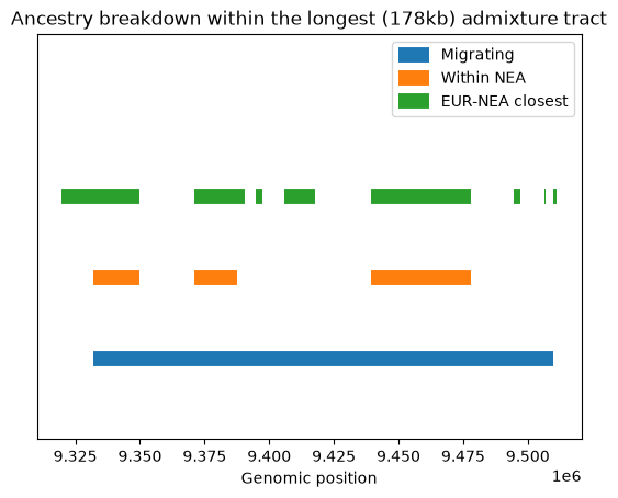
As we go back in time, the single 178kb admixture tract (in blue) breaks down, with some regions coalescing in the Neanderthal population (orange) and some not. Although quite a lot of the tract supports grouping Eurasians with Neanderthals (green), substantial chunks of the admixed (blue) tract do not map onto the green tracts, and therefore must support one of the two other topologies (African+Neanderthal or African+Eurasian). These must be due to ILS.

The green signal, which is a measure of the local tree topology and which is the primary signal that can be extracted from mutational data, is therefore not a very reliable guide to which regions of the genome have passed through the admixed route. In other words, admixed tracts are likely to be hard to detect simply from the distribution of mutations.

Locating mutations

We might be interested in finding the population in which mutations arose. For this, we first need to impose some mutations on the tree sequence using msprime.sim_mutations().

ts = msprime.sim_mutations(ts, rate=1e-8, random_seed=25)  # rate in /bp/gen

Now we work out which population the mutation occurred in, from the times of the mutation and the migration events. The following function takes a simple approach, first gathering the migrations for each node into a list then sequentially examining each migration that affects the mutation’s node and intersects with the site position. Because we know that the migration records are sorted in increasing time order, we can simply apply the effects of each migration while the migration record’s time is less than the time of the mutation. At the end of this process, we then return the computed mapping of mutation IDs to the populations in which they arose.

def get_mutation_population(ts):
    node_migrations = collections.defaultdict(list)
    for migration in ts.migrations():
        node_migrations[migration.node].append(migration)
    mutation_population = np.zeros(ts.num_mutations, dtype=int)
    for tree in ts.trees():
        for site in tree.sites():
            for mutation in site.mutations:                
                mutation_population[mutation.id] = tree.population(mutation.node)
                for mig in node_migrations[mutation.node]:
                    # Stepping through all migations will be inefficient for large 
                    # simulations. Should use an interval tree (e.g. 
                    # https://pypi.python.org/pypi/intervaltree) to find all 
                    # intervals intersecting with site.position.
                    if mig.left <= site.position < mig.right:
                        # Note that we assume that we see the migration records in 
                        # increasing order of time!
                        if mig.time < mutation.time:
                            assert mutation_population[mutation.id] == mig.source
                            mutation_population[mutation.id] = mig.dest
    return mutation_population

mutation_population = get_mutation_population(ts)

We can plot a fraction of the tree sequence (say the first 25kb) using styling to colour both mutations and nodes by their population:

time_units = 1000 / 25  # Conversion factor for kya to generations

colour_map = {0: "red", 1: "blue", 2: "green"}
css = ".y-axis .tick .grid {stroke: #CCCCCC} .y-axis .tick .lab {font-size: 85%}"
css += "".join([f".node.p{k} > .sym {{fill: {col}}}" for k, col in colour_map.items()])
css += "".join([
    f".mut.m{k} .sym {{stroke: {colour_map[v]}}} "
    f".mut.m{k} .lab {{fill: {colour_map[v]}}} "
    for k, v in enumerate(mutation_population)])
y_ticks = {0: "0", 30: "30", 50: "Introgress", 70: "Eur origin", 300: "Nea origin", 1000: "1000"}
y_ticks = {y * time_units: lab for y, lab in y_ticks.items()}
ts.draw_svg(
    size=(1200, 500),
    x_lim=(0, 25_000),
    time_scale="log_time",
    node_labels = {0: "Af", 1: "Eu", 2: "Ne"},
    y_axis=True,
    y_label="Time (kya)",
    x_label="Genomic position (bp)",
    y_ticks=y_ticks,
    y_gridlines=True,
    style=css,
)

The depth of the trees indicates that most coalescences occur well before the origin of Neanderthals, and are thus instances of ILS. Moreover, most mutations on the trees are red, indicating they occurred in the African population, although a few are blue (Eurasian origin) or green (Neanderthal origin). A more comprehensive approach might simply count the number of (say) mutations originating in Neanderthals:

import dataclasses
print(
    f"% of muts from Neanderthals: {np.sum(mutation_population==2)/ts.num_mutations*100:.2f}%")

% of muts from Neanderthals: 12.90%

This seems high because it includes all the mutations that original in Neanderthals that are only found in the Neanderthal genome (and not e.g. in the Eurasian sample). In real datasets these are usually removed, to leave only those mutations that have been introgressed from Neanderthals into modern humans. The percentage of introgressed Neanderthal mutations seen in modern humans is much smaller:

#  NOTE: we shouldn't need to mess with metadata to save mutation information once we can
#  simplify a tree sequence with migrations, see https://github.com/tskit-dev/tskit/issues/20
import tskit
tables = ts.dump_tables()
tables.mutations.clear()
tables.mutations.metadata_schema = tskit.MetadataSchema({"codec":"json"})
for p, row in zip(mutation_population, ts.tables.mutations):
    tables.mutations.append(dataclasses.replace(row, metadata={"pop":int(p)}))   
tables.migrations.clear()
tables.simplify([0, 1])
extant_ts = tables.tree_sequence()
num_introgressed_muts = np.sum([1 for m in extant_ts.mutations() if m.metadata['pop']==2])
print(
    f"% Neanderthal muts in moderns: {num_introgressed_muts/extant_ts.num_mutations*100:.2f}%")

% Neanderthal muts in moderns: 0.28%

So in this model, of the mutations in the ~2% of the Neanderthal genome contained in extant Eurasians, the vast majority happened in the ancestral African population. Only about 1 in 7 actually mutated in Neanderthals themselves.